Redes Neuronales Informadas en Física (PINNs)

Oscilador armónico amortiguado

Blog para explorar la solución al oscilador armónico amortiguado

Basado en la explicación de Ben Moseley

Vamos a explorar cómo crear una PINN con PyTorch para el problema

\[ m \dfrac{d^2 x}{d t^2} + \mu \dfrac{d x}{d t} + kx = 0~, \]

con condiciones iniciales

\[ x(0) = 1~~,~~\dfrac{d x}{d t} = 0~. \]

Vamos a concentrarnos en el estado sub-atenuado donde

\[ \delta < \omega_0~,~~~~~\mathrm{with}~~\delta = \dfrac{\mu}{2m}~,~\omega_0 = \sqrt{\dfrac{k}{m}}~. \]

En este caso la solución exacta es

\[ x(t) = e^{-\delta t}(2 A \cos(\phi + \omega t))~,~~~~~\mathrm{with}~~\omega=\sqrt{\omega_0^2 - \delta^2}~. \]

from PIL import Image

import numpy as np
import torch
import torch.nn as nn
import matplotlib.pyplot as plt
import os

def save_gif_PIL(outfile, files, fps=5, loop=0):
    "Helper function for saving GIFs"
    imgs = [Image.open(file) for file in files]
    imgs[0].save(fp=outfile, format='GIF', append_images=imgs[1:], save_all=True, duration=int(1000/fps), loop=loop)

def plot_result(x,y,x_data,y_data,yh,xp=None):
    "Pretty plot training results"
    plt.figure(figsize=(8,4))
    plt.plot(x,y, color="grey", linewidth=2, alpha=0.8, label="Solución exacta")
    plt.plot(x,yh, color="tab:blue", linewidth=4, alpha=0.8, label="Predicción de la red")
    plt.scatter(x_data, y_data, s=60, color="tab:orange", alpha=0.4, label='Datos de entrenamiento')
    if xp is not None:
        plt.scatter(xp, -0*torch.ones_like(xp), s=60, color="tab:green", alpha=0.4, 
                    label='Puntos de colocación')
    l = plt.legend(loc=(1.01,0.34), frameon=False, fontsize="large")
    plt.setp(l.get_texts(), color="k")
    plt.xlim(-0.05,2)
    plt.ylim(-1.1, 1.1)
    plt.title(f"Pasos de entrenamiento: {i}",fontsize="xx-large",color="k")
    # plt.axis("off")
    
def oscillator(d, w0, x):
    """Defines the analytical solution to the 1D underdamped harmonic oscillator problem. 
    Equations taken from: https://beltoforion.de/en/harmonic_oscillator/"""
    assert d < w0
    w = np.sqrt(w0**2-d**2)
    phi = np.arctan(-d/w)
    A = 1/(2*np.cos(phi))
    cos = torch.cos(phi+w*x)
    sin = torch.sin(phi+w*x)
    exp = torch.exp(-d*x)
    y  = exp*2*A*cos
    return y

class FCN(nn.Module):
    "Define una red neuronal completamente conectada"
    
    def __init__(self, N_INPUT, N_OUTPUT, N_HIDDEN, N_HIDDEN_LAYERS):
        super().__init__()
        
        activation = nn.Tanh
        layers = [nn.Linear(N_INPUT, N_HIDDEN), activation()]
        for _ in range(N_HIDDEN_LAYERS - 1):
            layers += [nn.Linear(N_HIDDEN, N_HIDDEN), activation()]
        layers += [nn.Linear(N_HIDDEN, N_OUTPUT)]
        
        self.net = nn.Sequential(*layers)
        
    def forward(self, x):
        return self.net(x)

Generamos datos

m = 1 # masa
k = 100 # constante del resorte
mu = 1 # coeficiente de amortiguacion

d = mu/2*m
w0 = np.sqrt(k/m)

# Solución analítica en el dominio (0,2)
t = torch.linspace(0,2,500).view(-1,1)
x = oscillator(d, w0, t).view(-1,1)
print(t.shape, x.shape)

# Elegimos puntos de entrenamiento, espaciados cada 20 puntos, para t menor a 1
t_data = t[0:241:20]
x_data = x[0:241:20]
print(t_data.shape, x_data.shape)

plt.figure()
plt.plot(t, x, label="Solución exacta")
plt.scatter(t_data, x_data, color="tab:orange", label="Datos observados")
plt.legend()
plt.xlabel("Tiempo (t)")
plt.ylabel("Posición x(t)")
plt.show()

torch.Size([500, 1]) torch.Size([500, 1])
torch.Size([13, 1]) torch.Size([13, 1])

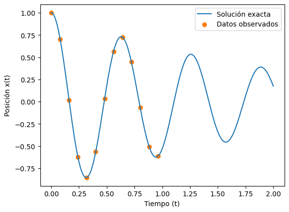
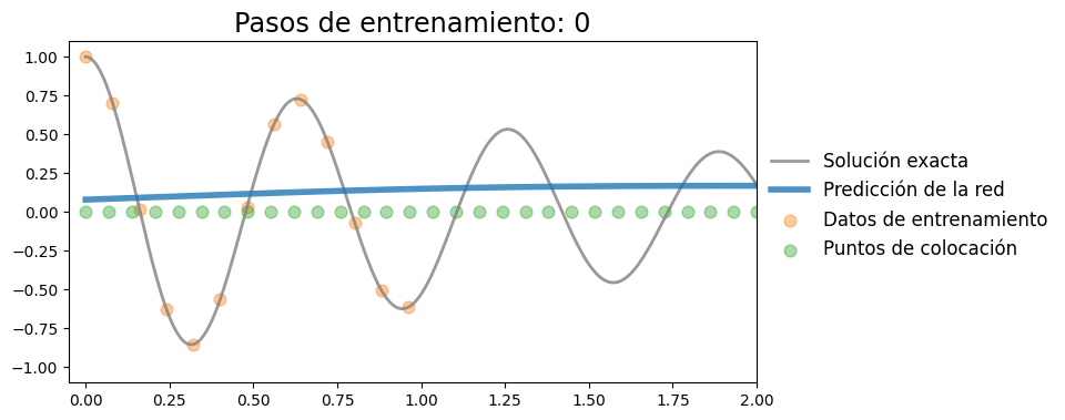
t_data e y_data contiene 10 puntos donde hemos observado la trayectoria de este oscilador

torch.manual_seed(2)
model = FCN(N_INPUT=1, N_OUTPUT=1, N_HIDDEN=20, N_HIDDEN_LAYERS=3)
optimizer = torch.optim.Adam(model.parameters(), lr=0.001)
criterion = nn.MSELoss()
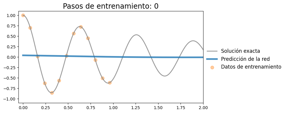
plotting_range = range(0,1001,50)
files = []
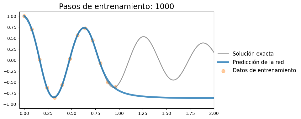
for i in range(1001):
    optimizer.zero_grad()
    x_pred = model(t_data)
    loss = criterion(x_pred, x_data)
    loss.backward()
    optimizer.step()
    
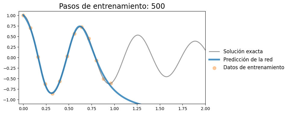
    if i in plotting_range:
        with torch.no_grad():
            x_pred = model(t).detach()
            
        plot_result(t, x, t_data, x_data, x_pred)
        file = f"figuras/nn_{i:08d}.png"
        plt.savefig(file, bbox_inches="tight", pad_inches=0.1, dpi=100, facecolor="white")
        files.append(file)
        
        if i%500 == 0:
            print(f"Iteración {i}, pérdida: {loss.item():.4f}")
            plt.show()
        else:
            plt.close("all")
            
save_gif_PIL("nn_training.gif", files, fps=5, loop=0)
        

---------------------------------------------------------------------------
FileNotFoundError                         Traceback (most recent call last)
Cell In[4], line 20
     16             x_pred = model(t).detach()
     17 
     18         plot_result(t, x, t_data, x_data, x_pred)
     19         file = f"figuras/nn_{i:08d}.png"
---> 20         plt.savefig(file, bbox_inches="tight", pad_inches=0.1, dpi=100, facecolor="white")
     21         files.append(file)
     22 
     23         if i%500 == 0:

File /opt/hostedtoolcache/Python/3.11.15/x64/lib/python3.11/site-packages/matplotlib/pyplot.py:1243, in savefig(*args, **kwargs)
   1240 fig = gcf()
   1241 # savefig default implementation has no return, so mypy is unhappy
   1242 # presumably this is here because subclasses can return?
-> 1243 res = fig.savefig(*args, **kwargs)  # type: ignore[func-returns-value]
   1244 fig.canvas.draw_idle()  # Need this if 'transparent=True', to reset colors.
   1245 return res

File /opt/hostedtoolcache/Python/3.11.15/x64/lib/python3.11/site-packages/matplotlib/figure.py:3490, in Figure.savefig(self, fname, transparent, **kwargs)
   3488     for ax in self.axes:
   3489         _recursively_make_axes_transparent(stack, ax)
-> 3490 self.canvas.print_figure(fname, **kwargs)

File /opt/hostedtoolcache/Python/3.11.15/x64/lib/python3.11/site-packages/matplotlib/backend_bases.py:2184, in FigureCanvasBase.print_figure(self, filename, dpi, facecolor, edgecolor, orientation, format, bbox_inches, pad_inches, bbox_extra_artists, backend, **kwargs)
   2180 try:
   2181     # _get_renderer may change the figure dpi (as vector formats
   2182     # force the figure dpi to 72), so we need to set it again here.
   2183     with cbook._setattr_cm(self.figure, dpi=dpi):
-> 2184         result = print_method(
   2185             filename,
   2186             facecolor=facecolor,
   2187             edgecolor=edgecolor,
   2188             orientation=orientation,
   2189             bbox_inches_restore=_bbox_inches_restore,
   2190             **kwargs)
   2191 finally:
   2192     if bbox_inches and restore_bbox:

File /opt/hostedtoolcache/Python/3.11.15/x64/lib/python3.11/site-packages/matplotlib/backend_bases.py:2040, in FigureCanvasBase._switch_canvas_and_return_print_method.<locals>.<lambda>(*args, **kwargs)
   2036     optional_kws = {  # Passed by print_figure for other renderers.
   2037         "dpi", "facecolor", "edgecolor", "orientation",
   2038         "bbox_inches_restore"}
   2039     skip = optional_kws - {*inspect.signature(meth).parameters}
-> 2040     print_method = functools.wraps(meth)(lambda *args, **kwargs: meth(
   2041         *args, **{k: v for k, v in kwargs.items() if k not in skip}))
   2042 else:  # Let third-parties do as they see fit.
   2043     print_method = meth

File /opt/hostedtoolcache/Python/3.11.15/x64/lib/python3.11/site-packages/matplotlib/backends/backend_agg.py:481, in FigureCanvasAgg.print_png(self, filename_or_obj, metadata, pil_kwargs)
    434 def print_png(self, filename_or_obj, *, metadata=None, pil_kwargs=None):
    435     """
    436     Write the figure to a PNG file.
    437 
   (...)    479         *metadata*, including the default 'Software' key.
    480     """
--> 481     self._print_pil(filename_or_obj, "png", pil_kwargs, metadata)

File /opt/hostedtoolcache/Python/3.11.15/x64/lib/python3.11/site-packages/matplotlib/backends/backend_agg.py:430, in FigureCanvasAgg._print_pil(self, filename_or_obj, fmt, pil_kwargs, metadata)
    425 """
    426 Draw the canvas, then save it using `.image.imsave` (to which
    427 *pil_kwargs* and *metadata* are forwarded).
    428 """
    429 FigureCanvasAgg.draw(self)
--> 430 mpl.image.imsave(
    431     filename_or_obj, self.buffer_rgba(), format=fmt, origin="upper",
    432     dpi=self.figure.dpi, metadata=metadata, pil_kwargs=pil_kwargs)

File /opt/hostedtoolcache/Python/3.11.15/x64/lib/python3.11/site-packages/matplotlib/image.py:1634, in imsave(fname, arr, vmin, vmax, cmap, format, origin, dpi, metadata, pil_kwargs)
   1632 pil_kwargs.setdefault("format", format)
   1633 pil_kwargs.setdefault("dpi", (dpi, dpi))
-> 1634 image.save(fname, **pil_kwargs)

File /opt/hostedtoolcache/Python/3.11.15/x64/lib/python3.11/site-packages/PIL/Image.py:2708, in Image.save(self, fp, format, **params)
   2706         fp = builtins.open(filename, "r+b")
   2707     else:
-> 2708         fp = builtins.open(filename, "w+b")
   2709 else:
   2710     fp = cast(IO[bytes], fp)

FileNotFoundError: [Errno 2] No such file or directory: 'figuras/nn_00000000.png'

Implementar PINN

Agregamos la pérdida física. Para esto, vamos a fijar los puntos de colocación

t_col = torch.linspace(0,2,30).unsqueeze(-1).requires_grad_()
t_col.shape

torch.Size([30, 1])

Supongamos que conocemos los parámetros del oscilador amortiguado, entonces podemos escribir el costo

def loss_fisica(model, t_col, mu, k, m):
    x_pred = model(t_col)
    x_t = torch.autograd.grad(x_pred, t_col, grad_outputs=torch.ones_like(x_pred), create_graph=True)[0] # calcula derivada primera
    x_tt = torch.autograd.grad(x_t, t_col, grad_outputs=torch.ones_like(x_t), create_graph=True)[0]  # calcula derivada segunda
    return torch.mean((m * x_tt + mu * x_t + k * x_pred)**2)
    
torch.manual_seed(3)
model = FCN(1, 1, 32, 3)
optimizer = torch.optim.Adam(model.parameters(), lr=0.001)
criterion = nn.MSELoss()
plotting_range = range(0,10001,100)
files = []
for i in range(10001):
    optimizer.zero_grad()
    x_pred = model(t_data)
    loss = criterion(x_pred, x_data)
    loss_f = loss_fisica(model, t_col, mu, k, m)
    loss_total = loss + 1e-4*loss_f
    loss_total.backward()
    optimizer.step()
    
    if i in plotting_range:
        with torch.no_grad():
            x_pred = model(t).detach()
            
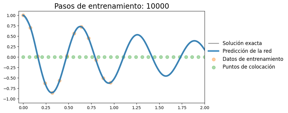
        plot_result(t, x, t_data, x_data, x_pred, xp=t_col.detach())
        file = f"figuras/pinn_{i:08d}.png"
        plt.savefig(file, bbox_inches="tight", pad_inches=0.1, dpi=100, facecolor="white")
        files.append(file)
        
        if i%2000 == 0:
            print(f"Iteración {i}, pérdida: {loss.item():.5f}")
            plt.show()
        else:
            plt.close("all")
            
save_gif_PIL("pinn_training.gif", files, fps=5, loop=0)

Iteración 0, pérdida: 0.38400

Iteración 2000, pérdida: 0.00007

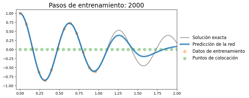
Iteración 4000, pérdida: 0.00002

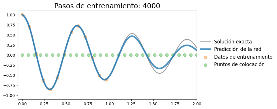
Iteración 6000, pérdida: 0.00000

Iteración 8000, pérdida: 0.00000

Iteración 10000, pérdida: 0.00000

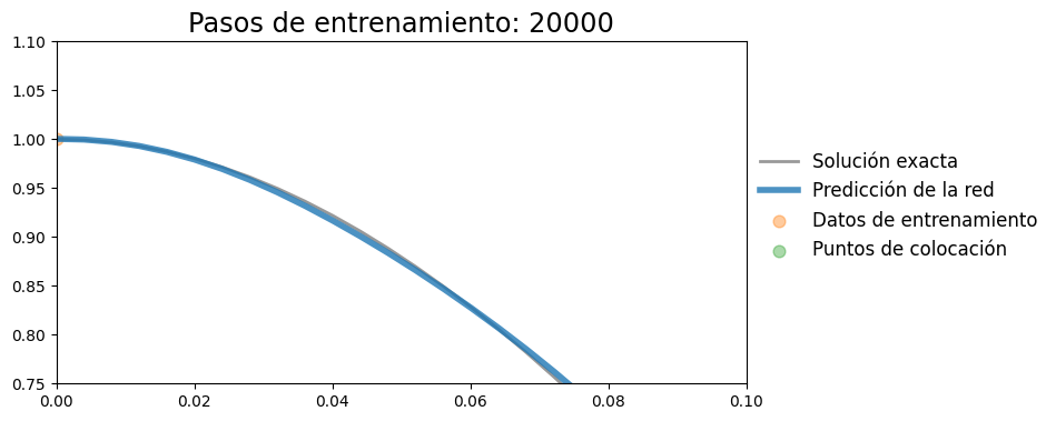
Agregar perdida de condicion inicial

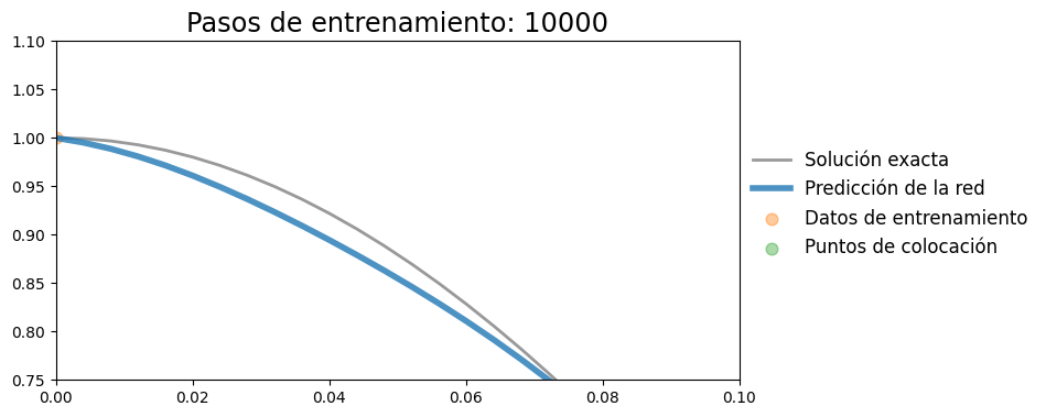
plot_result(t, x, t_data, x_data, x_pred, xp=t_col.detach())
plt.xlim(0,0.1)
plt.ylim(0.75,1.1)

(0.75, 1.1)

def loss_CI(model, t):
    x_pred = model(t)
    x_t = torch.autograd.grad(x_pred, t, grad_outputs=torch.ones_like(x_pred), create_graph=True)[0]
    return torch.mean((x_t)**2 + (x_pred-1)**2)

torch.manual_seed(3)
model = FCN(1, 1, 32, 3)
optimizer = torch.optim.Adam(model.parameters(), lr=0.001)
criterion = nn.MSELoss()
plotting_range = range(0,10001,2000)
files = []
for i in range(10001):
    optimizer.zero_grad()
    x_pred = model(t_data)
    loss = criterion(x_pred, x_data)
    loss_f = loss_fisica(model, t_col, mu, k, m)
    t0 = torch.tensor([[0.0]], requires_grad=True)
    loss_ci = loss_CI(model, t0)
    loss_total = loss + 1e-4*loss_f + 1e-4*loss_ci
    loss_total.backward()
    optimizer.step()
    
with torch.no_grad():
    x_pred = model(t).detach()
    
plot_result(t, x, t_data, x_data, x_pred, xp=t_col.detach())
plt.show()

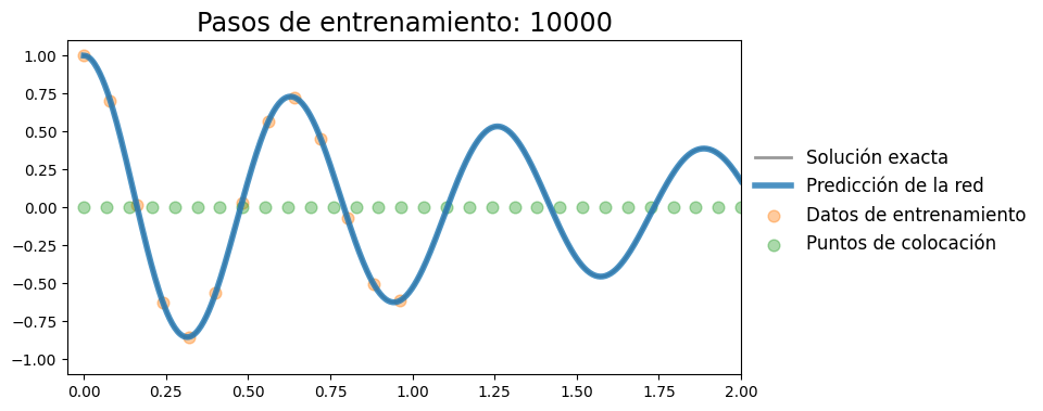
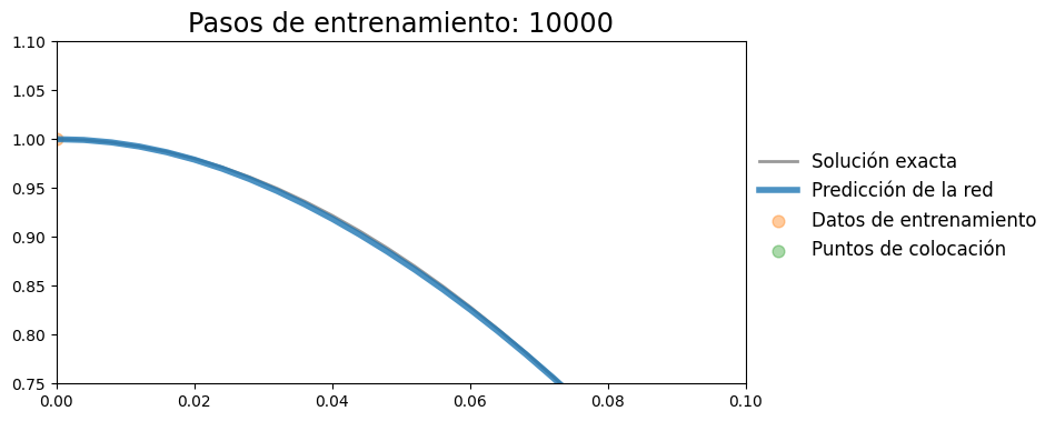
Vemos que la condición inicial se cumple relativamente bien, tanto en el valor como en la derivada

plot_result(t, x, t_data, x_data, x_pred, xp=t_col.detach())
plt.xlim(0,0.1)
plt.ylim(0.75,1.1)

(0.75, 1.1)

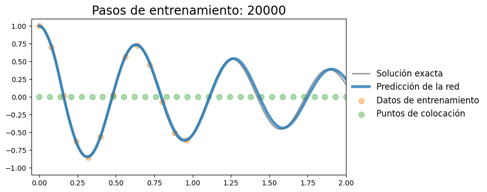
Inferencia: Deducción de parámetros

Supongamos que ahora no conocemos los parametros \(m\), \(k\), y \(\mu\) y quisieramos encontrarlos

k_raw = torch.nn.Parameter(torch.tensor([80.0], requires_grad = True))
mu_raw = torch.nn.Parameter(torch.tensor([2.0], requires_grad = True))

def positive(x):
    return torch.nn.functional.softplus(x)



torch.manual_seed(3)
model = FCN(1, 1, 32, 3)
optimizer = torch.optim.Adam(list(model.parameters()) + [k_raw, mu_raw], lr=0.001)
criterion = nn.MSELoss()
plotting_range = range(0,20001,2000)
files = []

for i in range(20001):
    optimizer.zero_grad()
    x_pred = model(t_data)
    loss = criterion(x_pred, x_data)
    
    k_par = positive(k_raw)
    mu_par = positive(mu_raw)
    loss_f = loss_fisica(model, t_col, mu_par, k_par, m)
    t0 = torch.tensor([[0.0]], requires_grad=True)
    loss_ci = loss_CI(model, t0)
    loss_total = loss + 1e-3*loss_f + 1e-2*loss_ci
    loss_total.backward()
    optimizer.step()
    if i%1000==0:
        print(f"Iteración {i}, pérdida: {loss.item():.6f}, k: {k_par.item():.4f}, mu: {mu_par.item():.4f}")
    
with torch.no_grad():
    x_pred = model(t).detach()
    
plot_result(t, x, t_data, x_data, x_pred, xp=t_col.detach())
plt.show()

Iteración 0, pérdida: 0.384004, k: 80.0000, mu: 2.1269
Iteración 1000, pérdida: 0.018542, k: 80.4644, mu: 2.2170
Iteración 2000, pérdida: 0.012968, k: 81.3869, mu: 2.2617
Iteración 3000, pérdida: 0.009333, k: 82.3507, mu: 1.9060
Iteración 4000, pérdida: 0.008665, k: 83.2601, mu: 1.8954
Iteración 5000, pérdida: 0.007905, k: 84.1714, mu: 1.8859
Iteración 6000, pérdida: 0.006939, k: 85.0658, mu: 1.8481
Iteración 7000, pérdida: 0.006543, k: 85.9220, mu: 1.7386
Iteración 8000, pérdida: 0.006028, k: 86.7210, mu: 1.6134
Iteración 9000, pérdida: 0.003981, k: 87.6295, mu: 1.4964
Iteración 10000, pérdida: 0.003224, k: 88.6279, mu: 1.4095
Iteración 11000, pérdida: 0.003390, k: 89.6316, mu: 1.3307
Iteración 12000, pérdida: 0.002027, k: 90.6089, mu: 1.2616
Iteración 13000, pérdida: 0.001459, k: 91.5560, mu: 1.2014
Iteración 14000, pérdida: 0.001227, k: 92.4709, mu: 1.1522
Iteración 15000, pérdida: 0.000937, k: 93.3549, mu: 1.1121
Iteración 16000, pérdida: 0.000735, k: 94.2101, mu: 1.0782
Iteración 17000, pérdida: 0.001067, k: 95.0376, mu: 1.0492
Iteración 18000, pérdida: 0.000356, k: 95.8191, mu: 1.0282
Iteración 19000, pérdida: 0.000230, k: 96.5503, mu: 1.0113
Iteración 20000, pérdida: 0.000295, k: 97.2126, mu: 1.0003

plot_result(t, x, t_data, x_data, x_pred, xp=t_col.detach())
plt.xlim(0,0.1)
plt.ylim(0.75,1.1)

(0.75, 1.1)